-
Book
-
Author
-
Contents
-
Libraries
-
Graphics
-
Programs
<
>
|
The book is devoted to the general field of numerical programming, with emphasis on methods specific to computational physics and engineering.
The book is addressed to advanced undergraduate and graduate students in natural sciences and engineering, with the aim of being suited as curriculum material for a one- or two-semester course in numerical programming based on Python or C/C++. The book may also be used for independent study or as a reference material beyond academic studies. It may be useful, for instance, as an introductory text for researchers preparing to engage in scientific computing, or engineers needing effective numerical tools for applicative calculations. All the materials on this web site are released as 'open source', with the only request that the authorship and the book are mentioned. Please also visit the book's web site at CRC Press / Taylor & Francis Group. Feedback to the author is highly appreciated! |
|
I am Titus Adrian Beu, professor emeritus at the Faculty of Physics of the "Babeș-Bolyai" University from Cluj-Napoca, Romania.
I have been active in the broader field of computational physics for more than 40 years, both in research and academia. My research has been theoretical and computational in nature, covering a multitude of topics. These have evolved from Tokamak plasma and nuclear reactors in the 1980s, collision theory and molecular cluster spectroscopy in the 1990s, fullerenes and nanofluidics in the 2000s, to complex biomolecular systems of interest in drug delivery, in recent years. The development of complex computer codes has always been at the heart of all the research projects I have conducted. In parallel, I gave university lectures on general programming techniques and advanced numerical methods, computer simulation methods, and advanced molecular dynamics. The material covered in the book comes together from my research experience and the computational physics courses taught at the university. The core material has undergone a continuous process of distillation and reformulation over the years, following the evolution of modern programming concepts and technologies. I am happy to receive opinions, questions, requests,... Have fun reading the book and practicing numerical programming! titus,[email protected] |
|
1 Approximate Numbers
1.1 Sources of errors in numerical calculations 1.2 Absolute and relative errors 1.3 Representation of numbers 1.4 Significant digits 1.5 Errors of elementary operations 1.5.1 Error of a sum 1.5.2 Error of a difference 1.5.3 Error of a product 1.5.4 Error of a quotient References 2 Basic Programming Techniques 2.1 Programming concepts 2.2 Functions and parameters 2.3 Passing arguments to Python functions 2.4 Passing arguments to C/C++ functions 2.5 Arrays in Python 2.6 Dynamic array allocation in C/C++ 2.7 Basic matrix operations References 3 Elements of Scientific Graphics 3.1 The Tkinter package 3.2 The Canvas widget 3.2.1 Commonly used Canvas items 3.2.2 Methods for updating Canvas widgets 3.3 Simple Tkinter applications 3.4 Plotting functions of one variable 3.5 The graphics library graphlib.py 3.5.1 Auxiliary functions 3.5.2 Routines for plotting functions 3.5.3 Simple 3D rendering routines 3.5.4 Histograms 3.6 Creating plots in C++ using the library graphlib.py References 4 Sorting and Indexing 4.1 Introduction 4.2 Bubble sort 4.3 Insertion sort 4.4 Quicksort 4.5 Indexing and ranking 4.6 Implementations in C/C++ 4.7 Problems References 5 Evaluation of Functions 5.1 Evaluation of polynomials by Horner's scheme 5.2 Evaluation of analytic functions 5.3 Continued fractions 5.4 Orthogonal polynomials 5.5 Spherical harmonics. Associated Legendre functions 5.6 Spherical Bessel functions 5.7 Implementations in C/C++ 5.8 Problems References 6 Algebraic and Transcendental Equations 6.1 Root separation 6.2 Bisection method 6.3 Method of false position 6.4 Method of successive approximations 6.5 Newton's method 6.6 Secant method 6.7 Birge-Vieta method 6.8 Newton's method for systems of nonlinear equations 6.9 Implementations in C/C++ 6.10 Problems References 7 Systems of Linear Equations 7.1 Introduction 7.2 Gaussian elimination with backward substitution 7.3 Gauss-Jordan elimination 7.4 LU factorization 7.5 Inversion of triangular matrices 7.6 Cholesky factorization 7.7 Tridiagonal systems of linear equations 7.8 Block tridiagonal systems of linear equations 7.9 Complex matrix equations 7.10 Jacobi and Gauss-Seidel iterative methods 7.11 Implementations in C/C++ 7.12 Problems References 8 Eigenvalue problems 8.1 Introduction 8.2 Diagonalization of matrices by similarity transformations 8.3 Jacobi method 8.4 Generalized eigenvalue problems for symmetric matrices 8.5 Implementations in C/C++ 8.6 Problems References |
9 Modeling of Tabulated Functions
9.1 Interpolation and regression 9.2 Lagrange interpolation polynomial 9.3 Neville's interpolation method 9.4 Cubic spline interpolation 9.5 Linear regression 9.6 Multilinear regression models 9.7 Nonlinear regression. The Levenberg-Marquardt method 9.8 Implementations in C/C++ 9.9 Problems References 10 Integration of Functions 10.1 Introduction 10.2 Trapezoidal Rule; A Heuristic Approach 10.3 The Newton-Cotes Quadrature Formulas 10.4 Trapezoidal Rule 10.5 Simpson's Rule 10.6 Adaptive Quadrature Methods 10.7 Romberg's Method 10.8 Improper Integrals: Open Formulas 10.9 Midpoint Rule 10.10 Gaussian Quadratures 10.11 Multidimensional integration 10.12 Adaptive multidimensional integration 10.13 Implementations in C/C++ 10.14 Problems References 11 Monte Carlo Method 11.1 Introduction 11.2 Integration of functions 11.3 Importance sampling 11.4 Multidimensional integrals 11.5 Generation of random numbers 11.6 Implementations in C/C++ 11.7 Problems References 12 Ordinary Differential Equations 12.1 Introduction 12.2 Taylor series method 12.3 Euler's method 12.4 Runge-Kutta methods 12.5 Adaptive step size control 12.6 Methods for second-order ODEs 12.7 Numerov's method 12.8 Shooting methods for two-point problems 12.9 Finite-difference methods for linear two-point problems 12.10 Implementations in C/C++ 12.11 Problems References 13 Partial Differential Equations 13.1 Introduction 13.2 Boundary-value problems for elliptic differential equations 13.3 Initial-value problems for parabolic differential equations 13.3.1 Explicit finite-difference method 13.3.2 von Neumann stability analysis 13.3.3 Implicit finite-difference method 13.3.4 Crank-Nicolson method 13.3.5 Spatially variable diffusion coefficient 13.4 Time-dependent Schrödinger equation 13.5 Initial-value problems for hyperbolic differential equations 13.6 Implementations in C/C++ 13.7 Problems References A Dynamic array allocation in C/C++ B Basic operations with vectors and matrices C Embedding Python in C/C++ References D The numerical libraries numxlib.py and numxlib.h E The graphics library graphlib.py based on Tkinter F The C++ interface to the graphics library graphlib.py G List of programs by chapter Index |
The numerical libraries numxlib.py and numxlib.h
The partial numerical libraries developed along the chapters compose the general libraries numxlib.py and numxlib.h. The corresponding Python and C/C++ routines have identical names and functionalities. The only naming exception concerns the modules random1.py and random.h, and this is due to the existence of a standard Python module named random.py.
numxlib.h also includes memalloc.h, containing dynamic memory allocation routines for vectors and matrices in C/C+.
numxlib.h also includes memalloc.h, containing dynamic memory allocation routines for vectors and matrices in C/C+.
|
| ||||||||||||
numxlib.py Library of numerical methods for Python.
numxlib.h Library of numerical methods for C.
Component modules
sort.py / sort.h
Contain routines for sorting, indexing, and ranking numeric sequences:
BubbleSort - Sorts a numeric sequence using bubble sort.
InsertSort - Sorts a numeric sequence by direct insertion.
QuickSort - Sorts a numeric sequence using Quicksort.
Index - Indexes a numeric sequence by direct insertion.
Rank - Ranks a numeric sequence based on the array of indexes.
Index2 - Performs the indexing of two correlated arrays by direct insertion.
specfunc.py / specfunc.h
Contain routines for evaluating special functions:
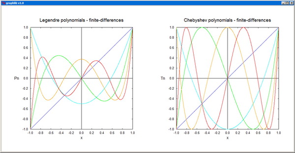
Chebyshev - Evaluates Chebyshev polynomials of the first kind and their derivatives using the recurrence relation.
Legendre - Evaluates Legendre polynomials and their derivatives using the recurrence relation.
aLegendre - Evaluates associated Legendre functions.
Laguerre - Evaluates Laguerre polynomials and their derivatives using the recurrence relation.
aLaguerre - Evaluates associated Laguerre polynomials.
Hermite - Evaluates Hermite polynomials and their derivatives using the recurrence relation.
SpherY - Evaluates the real and imaginary parts of spherical harmonics.
SBessy - Evaluates spherical Neumann functions.
SBessj - Evaluates spherical Bessel functions.
roots.py / roots.h
Contain routines for determining real roots of real functions:
Bisect - Determines a real root of a function by the bisection method.
FalsPos - Determines a real root of a function by the false position method.
Iter - Determines a real root of a function by the method of successive approximations.
Newton - Determines a real root of a function by the Newton-Raphson method using the analytical derivative.
NewtonNumDrv - Determines a real root of a function by the Newton-Raphson method using the numerical derivative.
Secant - Determines a real root of a function by the secant method.
BirgeVieta - Determines real roots of polynomials by the Birge-Vieta method.
Jacobian - Calculates the Jacobian of a system of multidimensional functions using central finite differences.
NewtonSys - Solves a system of nonlinear equations by Newton's method.
linsys.py / linsys.py
Contain routines for solving systems of linear equations:
Gauss - Solves a matrix equation by Gaussian elimination with partial pivoting.
GaussJordan0 - Solves a matrix equation by Gauss-Jordan elimination with partial pivoting.
GaussJordan1 - Solves a matrix equation by Gauss-Jordan elimination with partial pivoting and matrix inversion.
GaussJordan - Solves a matrix equation by Gauss-Jordan elimination with complete pivoting and matrix inversion.
LUFactor - Performs LU factorization of a matrix by Doolittle's method.
LUSystem - Solves a linear system using the LU decomposition of its matrix.
MatInv - Performs matrix inversion using LU factorization.
MatTriInv - Inverts a triangular matrix.
Cholesky - Performs the Cholesky factorization of a symmetric positive-definite matrix.
CholeskySys - Solves a positive-definite linear system using the Cholesky decomposition of its matrix.
MatSymInv - Inverts a positive-definite matrix using the Cholesky factorization.
TriDiagSys - Solves a linear system with tridiagonal matrix.
GaussSeidel - Solves a system of linear equations by the Gauss-Seidel method.
eigsys.p y / eigsys.h
Contain routines for solving eigenvalue problems:
Jacobi Solves an eigenvalue problem for a real symmetric matrix using the Jacobi method.
EigSym - Solves a generalized eigenvalue problem for real symmetric (positive-definite) matrices.
EigSort - Sorts a set of eigenvalues and eigenvectors according to the eigenvalues.
modfunc.py / modfunc.h
Contain routines for modeling tabular dependences by interpolation or regression:
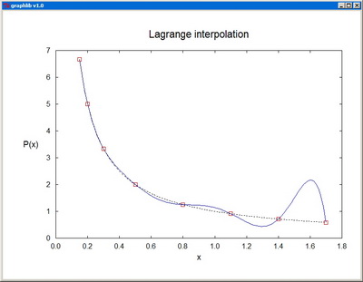
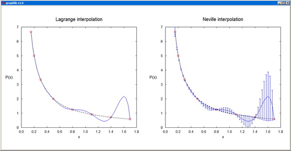
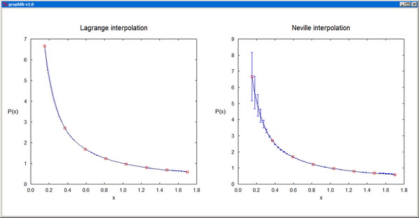
Lagrange - Evaluates the Lagrange interpolating polynomial for a set of data points.
Neville - Evaluates the Lagrange interpolating polynomial by Neville's method.
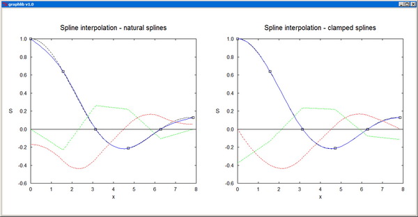
Spline - Performs cubic spline interpolation.
LinFit - Performs linear regression on a set of data points.
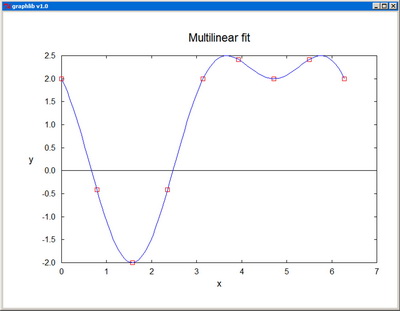
MultiFit - Performs multilinear regression on a set of data points.
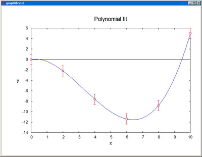
PolFit - Performs polynomial regression on a set of data points.
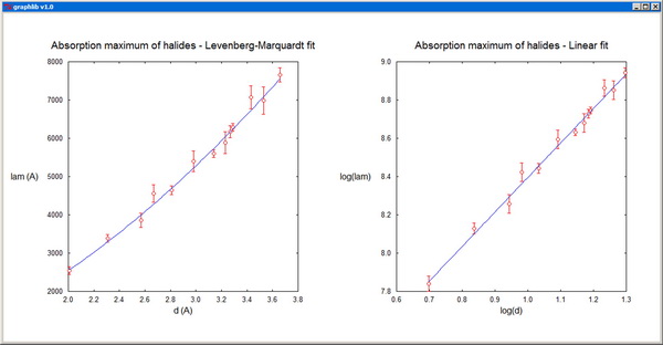
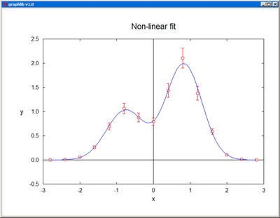
MarqFit - Performs nonlinear regression based on the Levenberg-Marquardt method.
integral.py / integral.h
Contain 1D and 3D integrators for real functions with real variables:
qTrapz - Function integrator based on the trapezoidal rule.
qSimpson - Function integrator based on Simpson's rule.
qTrapzCtrl - Adaptive integrator based on the trapezoidal rule.
qSimpsonCtrl - Adaptive integrator based on Simpson's rule.
qRomberg - Adaptive integrator based on Romberg's method.
qImprop1 - Adaptive integrator for improper integrals of the first kind (with infinite limits).
qImprop2 - Adaptive integrator for improper integrals of the second kind (with singular integrable limits).
qMidPoint - Adaptive integrator based on the midpoint rule.
xGaussLeg - Generates abscissas and weights for Gauss-Legendre quadratures.
qGaussLeg - Gauss-Legendre integrator.
xGaussLag - Generates abscissas and weights for Gauss-Laguerre quadratures.
qGaussLag - Gauss-Laguerre integrator.
qTrapz3D - 3D integrator based on the trapezoidal rule.
xSimpson - Generates integration points and weights for Simpson's rule.
qSimpson3D - 3D integrator based on Simpson's rule.
qGaussLeg3D - 3D integrator based on Gaussian quadratures.
qSimpsonAng - Integrator in spherical angular coordinates based on Simpson's rule.
qSimpsonSph - Integrator in spherical coordinates based on Simpson's rule.
qGaussSph - Integrator in spherical coordinates based on Gaussian quadratures.
qSimpsonCyl - Integrator in cylindrical coordinates based on Simpson's rule.
random1.py / random.h
Contain routines for generating pseudorandom numbers:
randLCG1 - Linear congruential random number generator based on specifications from Press et al. 2002.
randLCG2 - Linear congruential random number generator based on specifications from Rapaport 2004.
randMCG - Multiply-with-Carry random number generator based on specifications of George Marsaglia.
randNrm - Generates random numbers with normal distribution based on the central limit theorem.
randNrm2 - Returns two random numbers with normal distribution.
randMet - Random number generator based on the Metropolis method.
ode.py / ode.h
Contain routines for solving systems of ordinary differential equations:
Euler - Euler propagator for systems of first-order ODEs.
EulerPC - Euler predictor-corrector propagator for systems of first-order ODEs.
RungeKutta - Fourth-order Runge-Kutta solver for Cauchy problems for systems of first-order ODEs.
RKadapt - Adaptive ODE solver using step-halving and the Runge-Kutta method.
RKFehlberg - Adaptive ODE solver based on the Runge-Kutta-Fehlberg method.
Euler1 - Euler propagator for a second-order ODE.
EulerCromer1 - Euler-Cromer propagator for a second-order ODE.
Verlet1 - Verlet propagator for a second-order ODE.
Euler2 - Euler propagator for a system of second-order ODEs.
EulerCromer - Euler-Cromer propagator for a system of second-order ODEs.
Verlet2 - 2D velocity Verlet propagator for a single particle.
Verlet - Velocity Verlet propagator for a system of particles in interaction.
EulerCromerQM - Euler-Cromer integrator for the 1D Schrödinger equation.
Numerov - Numerov integrator for the 1D Schrödinger equation.
Propag - Propagates the solution of a second-order ODE on a regular mesh using the Euler-Cromer method.
Shoot - Solves a two-point boundary-value problem for a second-order ODE using the shooting method.
ShootQM - Solves the 1D Schrödinger equation using the shooting method.
Bilocal - Linear bilocal problem solver based on the finite-difference method.
pde.py / pde.h
Contain routines for solving partial differential equations:
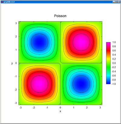
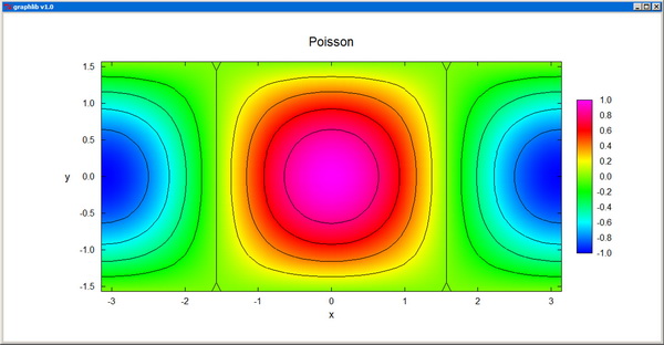
Poisson0 - Solver for the 2D Poisson equation in Cartesian coordinates with Dirichlet boundary conditions.
PoissonXY - Solver for the 2D Poisson equation in Cartesian coordinates with arbitrary boundary conditions.
Poisson2D - Solver for the 2D Poisson equation in Cartesian coordinates on an irregular domain.
PropagFTCS - Explicit forward-time central-space propagator for the diffusion equation.
PropagBTCS - Implicit backward-time central-space propagator for the diffusion equation.
PropagCN - Crank-Nicolson propagator for the diffusion equation.
PropagDiff - Crank-Nicolson propagator for the diffusion equation with variable diffusion coefficient.
PropagQTD - Crank-Nicolson propagator for the Schrödinger equation based on tridiagonal solver.
PropagQGS - Crank-Nicolson propagator for the Schrödinger equation using the Gauss-Seidel method.
PropagWave - Explicit forward-time central-space propagator for the classical wave equation.
utils.py / utils.h
Contain utility routines:
Nint - Returns the nearest integer to its real-type argument.
Sign - Transfers the sign of its second argument onto the absolute value of the first argument.
Magn - Returns the order of magnitude of its argument as a power of 10.
Index - Indexes a numeric sequence by direct insertion
Auxiliary libraries
memalloc.h
Contains functions for dynamic memory allocation of vectors and matrices in C:
Vector, FreeVector - Allocate/deallocate a double vector with indices in the range [imin,imax].
Matrix, FreeMatrix - Allocate/deallocate a double matrix, with row and column indices in the range [imin,imax] x [jmin,jmax].
IVector, FreeIVector - Allocate/deallocate an int vector with indices in the range [imin,imax].
IMatrix, FreeIMatrix - Allocate/deallocate an int matrix, with row and column indices in the range [imin,imax] x [jmin,jmax].
CVector, FreeCVector - Allocate/deallocate a complex vector with indices in the range [imin,imax].
CMatrix, FreeCMatrix - Allocate/deallocate a complex matrix, with row and column indices in the range [imin,imax] x [jmin,jmax].
coords.py / coords.h
Contain routines for transforming the coordinates of systems of particles:
MovetoCM - Moves a system of n particles to the CM system.
PrincipalAxes - Rotates a set of n particles to the system of principal axes.
Contain routines for transforming the coordinates of systems of particles:
MovetoCM - Moves a system of n particles to the CM system.
PrincipalAxes - Rotates a set of n particles to the system of principal axes.
elemfunc.py / elemfunc.h
Contain routines for evaluating elementary functions:
Poly - Evaluates a real polynomial using Horner's scheme.
PolyDerive - Returns the coefficients of the derivative of a real polynomial.
PolyDivide - Returns the coefficients of the division of a real polynomial by a binomial (x-x0).
Contain routines for evaluating elementary functions:
Poly - Evaluates a real polynomial using Horner's scheme.
PolyDerive - Returns the coefficients of the derivative of a real polynomial.
PolyDivide - Returns the coefficients of the division of a real polynomial by a binomial (x-x0).
matutil.py / matutil.h
Contain utility routines for basic operations with vectors and matrices:
MatRead - Reads from the keyboard the elements of matrix.
MatPrint - Prints the elements of a matrix on the display.
MatPrintTrans - Prints the elements of a transposed matrix on the display.
MatZero - Zeros the elements of a matrix.
MatCopy - Copies a matrix into another matrix.
MatTrans - Replaces a square matrix by its transpose.
MatDiff - Returns the difference of two matrices.
MatProd - Returns the product of two matrices.
MatPow - Returns a power of a square matrix.
MatNorm - Returns the max norm of a matrix.
VecPrint - Prints the elements of a vector on the display.
VecZero - Zeros the elements of a vector.
VecCopy - Copies a vector into another vector.
VecDiff - Returns the difference of two vectors.
VecNorm - Returns the 2-norm of a vector.
MatVecProd - Returns the product of matrix and a vector.
The graphics library grafxlib.py
The graphics library graphlib.py, accompanying the book was renamed grafxlib.py to avoid confusions with a recent standard module of Python. grafxlib.py is used throughout to produce runtime graphics both from Python and C/C++. The C/C++ applications can access grafxlib.py via the interface grafxlib.h.
grafxlib.py |
Graphics library for Python based on Tkinter. |
grafxlib.h |
C/C++ interface to the library grafxlib.py. |
|
| ||||||||||||
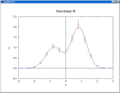
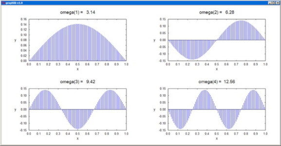
Sample plots
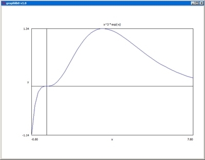
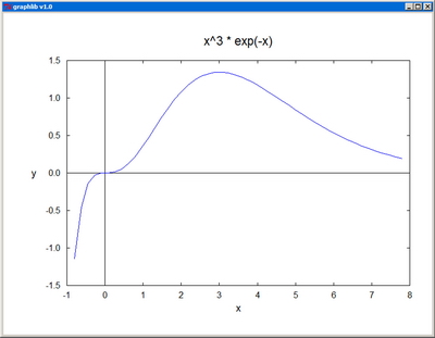
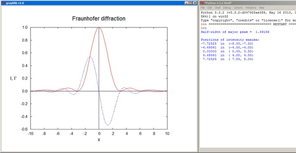
Simple example - plotting a function of one variable:
Python code:
C code:
To see all graphics applications, go to section Programs.
Structure of grafxlib.py
Auxiliary functions
Limits extends an arbitrary real interval so as to include an integer number of equal subintervals of length expressible as d x 10p, with d = 2, 5, or 10 and p integer. Output: xmin and xmax--adjusted values of, scale--scale factor (10p), nsigd--number of significant digits required to optimally represent the limits, nintv--resulting integer number of subintervals. Limits is typically called by Plot and MultiPlot to adjust the x and y user intervals for optimal labeling of the axes, by Contour to resize contour plots, and by ColorLegend to resize color legends.
FormStr determines the optimal labeling format for a given value x on the basis of previous output from Limits (scale factor scale and number of significant digits nsigd), and separates the mantissa in mant[] and the exponent of 10 in expn[].
ColorLegend and RGBcolors are used to display a color legend alongside a contour plot.
Routines for plotting functions
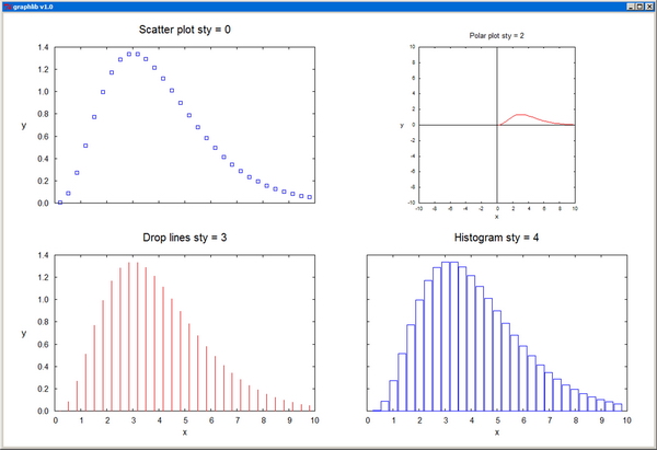
Plot plots a real function of one variable. The arrays x[] and y[] should contain the coordinates pairs of the representative points. The plot color is specified by the parameter col, and the corresponding arguments can be RGB colors or standard color names. The plot-style parameter sty can take one of the integer values: 0--scatter plot, 1--line plot, 2--polar plot, 3--drop lines, 4--histogram. fxmin, fxmax, fymin, fymax are the fractional limits of the plotting domain on the canvas. xtext, ytext, and title are the titles of the axes and of the whole graph. "None" as axis title inhibits the labeling of the axis altogether. The independent coordinate x[] is not supposed to vary monotonically, and this also enables the representation of cyclic functions.
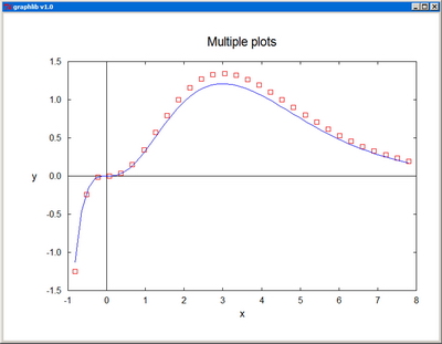
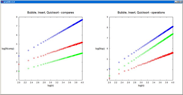
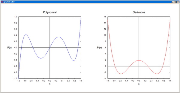
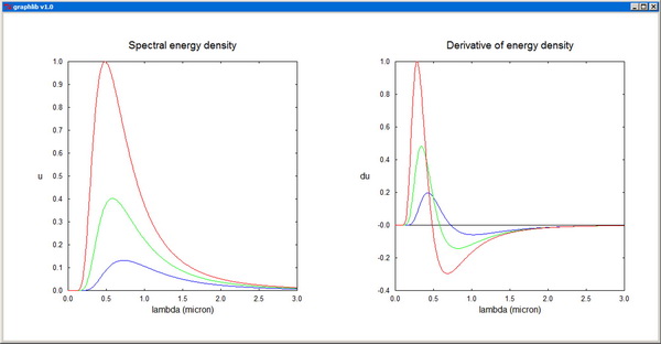
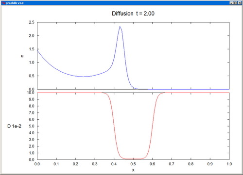
MultiPlot plots several functions of one variable on a single graph. The representative points of the nplot plots are contiguously packed in sequenced sets in the same vectors x[] and y[], with an additional array, n[], specifying the ending index for each set. sig[] is only used when error bars (sty[i]=4) are employed for at least one of the plots. col[] contains the colors of the individual plots and sty[] specifies the corresponding style parameters: 0--scatter plot, 1--line plot, -1--line plot with dashed line, 2--polar plot, -2--polar plot with dashed line, 3--drop lines, 4--error bars, -4--error bars and continuous line. For ioptx set to 0, the x-axis is resized automatically, while for nonzero ioptx, the axis is resized based on the provided user interval [xminp,xmaxp]. The y-axis is resized analogously, in accordance with the option iopty.
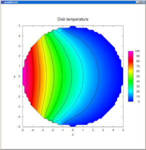
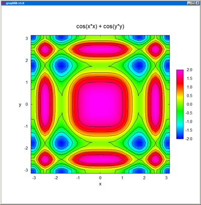
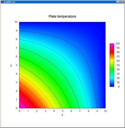
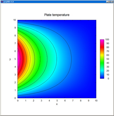
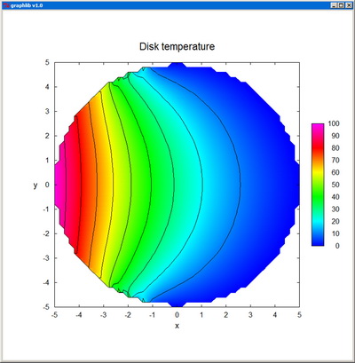
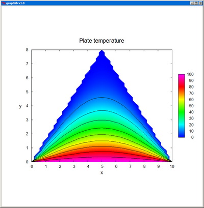
Contour creates the contour plot of a real function of two variables, defined in the domain [xmin,xmax] x [ymin,ymax] and specified by its values z[i][j] at the nx x ny nodes of a regular grid. The representation is confined to z-values between zmin and zmax.
Simple 3D rendering routines
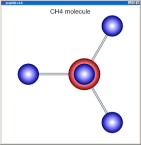
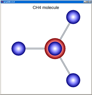
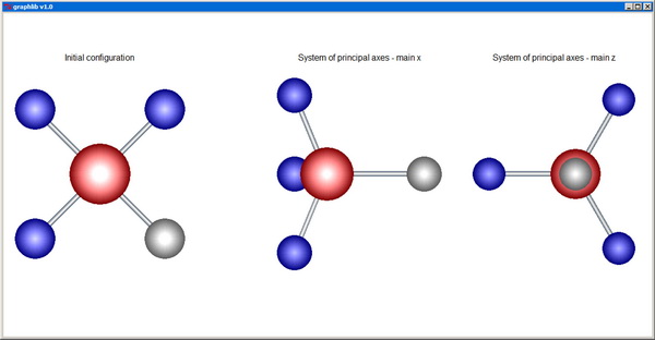
PlotParticles depicts systems of particles as spheres, optionally connected by cylindrical bonds. The input consists of the coordinate vectors x[], y[], and z[] of the centers of the n particles, their radii r[], and colors col[]. dmax is a cutoff distance beyond which the particles are no longer linked by bonds (with dmax set to 0, no bonds at all are depicted). The ioptx and iopty parameters control whether the x and y-axis, respectively, are to be sized automatically in order to reveal the entire structure (ioptx=0 and iopty=0), or, instead, the input user coordinates (xminp,xmaxp) and (yminp,ymaxp) are to be considered to crop the image.
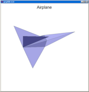
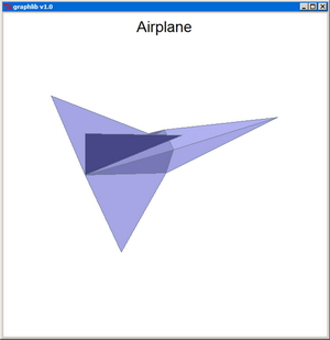
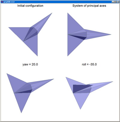
PlotStruct is a simple 3D rendering routine for structures specified by nodes and triangular surfaces defined between them. The input to PlotStruct consists of the coordinate vectors x[], y[], and z[] of the n nodes and the indexes ind1[], ind2[], and ind3[] of the nodes defining each of the n3 triangles.
PlotStruct is a simple 3D rendering routine for structures specified by nodes and triangular surfaces defined between them. The input to PlotStruct consists of the coordinate vectors x[], y[], and z[] of the n nodes and the indexes ind1[], ind2[], and ind3[] of the nodes defining each of the n3 triangles.
Histograms
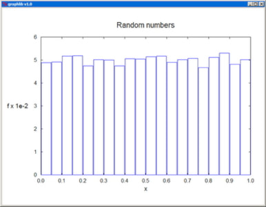
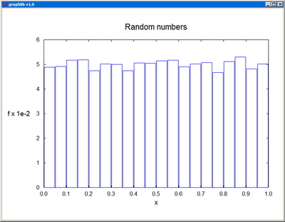
Histograms can be plotted using Plot with the style parameter sty=4. Before plotting a histogram, the data need to be binned. HistoBin is normally called in three successive modes:
- Initializing the histogram--defining the boundaries of the bins and zeroing the corresponding frequencies.
- Binning new observations--assigning them to the appropriate bins and incrementing the corresponding occurrence frequencies.
- Normalizing the histogram--dividing the frequencies by the total number of observations.
Creating plots in C/C++ using the library grafxlib.py
The C/C++ programs including the interface file grafxlib.h can seamlessly call with similar syntax the Python graphics functions defined in the module grafxlib.py. The proper functioning of grafxlib.h requires access to grafxlib.py (and to the therein imported module utils.py)) either by search path settings or by simply placing the three files in the same folder.
List of programs by chapter
The file names of the application programs contain the complete information on their location within the folder structure descending from the root folder /INP/. The general format of the file names is Pnn-name.py or Pnn-name.cpp, whereby nn indicates the chapter folder /INP/Chnn/ and the extension indicates the respective subfolder, that is, /INP/Chnn/Python/ or /INP/Chnn/C/.
A trailing "~" in their names, indicates updated versions of the files.
A trailing "~" in their names, indicates updated versions of the files.
2 Basic Programming Techniques
| Listing | File | Output | |
|---|---|---|---|
| 2.1 2.2 |
P02-Fact_global.py P02-Fact_global.cpp |
Factorial with global variables. | |
| 2.3 2.4 |
P02-Fact_comb.py P02-Fact_comb.cpp |
Combinations using a factorial function. | |
|
P02-Fact_recur.py P02-Fact_recur.cpp |
Factorial based on recursivity. | ||
| 2.7 2.9 2.10 |
P02-Swap~.py P02-Swap.c P02-Swap.cpp |
Returning swapped arguments from a function. | |
| 2.8 | P02-Swap_list~.py | Returning swapped list elements from a function. | |
| 2.18 2.19 |
P02-MatOp.py P02-MatOp.cpp |
Check of identity (A B)T = BT AT for random arrays A and B. |
| p02.zip | |
| File Size: | 4 kb |
| File Type: | zip |
3 Elements of Scientific Graphics
| p03.zip | |
| File Size: | 12 kb |
| File Type: | zip |
4 Sorting and Indexing
| p04.zip | |
| File Size: | 10 kb |
| File Type: | zip |
5 Evaluation of Functions
| p05.zip | |
| File Size: | 10 kb |
| File Type: | zip |
6 Algebraic and Transcendental Equations
| p06.zip | |
| File Size: | 14 kb |
| File Type: | zip |
7 Systems of Linear Equations
| Listing | File | Output | |
|---|---|---|---|
| 7.2 |
P07-Gauss.py P07-Gauss.cpp |
Solution of a linear system by Gaussian elimination. | |
| 7.6 |
P07-GaussJordan.py P07-GaussJordan.cpp |
Solution of a matrix equation by Gauss-Jordan elimination. | |
| 7.11 |
P07-MatInv.py P07-MatInv.cpp |
Check of matrix inversion based on LU factorization. | |
| 7.18 |
P07-TriDiagSys.py P07-TriDiagSys.cpp |
Solution of linear system with tridiagonal matrix by LU factorization. | |
|
P07-GaussSeidel.py P07-GaussSeidel.cpp |
Solution of linear system by the Gauss-Seidel method. | ||
| 7.21 7.22 |
P07-GaussJordan1.py P07-GaussJordan1.cpp |
Solution of a matrix equation by Gauss-Jordan elimination. | |
| 7.23 7.24 |
P07-LUFactor.py P07-LUFactor.cpp |
Solution of multiple linear systems by LU factorization. | |
| 7.25 |
P07-TriDiagSys1.py P07-TriDiagSys1.cpp |
Solution of system with tridiagonal matrix by LU factorization. | |
| 7.26 |
P07-MatDetIdent.py P07-MatDetIdent.cpp |
Check of identity for determinant of matrix product. | |
| 7.27 |
P07-MatInvIdent.py P07-MatInvIdent.cpp |
Check of identity for inverse of matrix product. | |
| 7.28 |
P07-MatSymInv.py P07-MatSymInv.cpp |
Inversion of symmetric positive-definite matrix by Cholesky factorization. | |
| 7.29 |
P07-Wavelet.py P07-Wavelet.cpp |
Solution of linear system for Daubechies D4 wavelet. |
| p07.zip | |
| File Size: | 14 kb |
| File Type: | zip |
8 Eigenvalue problems
| p08.zip | |
| File Size: | 11 kb |
| File Type: | zip |
9 Modeling of Tabulated Functions
| p09.zip | |
| File Size: | 40 kb |
| File Type: | zip |
10 Integration of Functions
| p10.zip | |
| File Size: | 17 kb |
| File Type: | zip |
11 Monte Carlo Method
| p11.zip | |
| File Size: | 18 kb |
| File Type: | zip |
12 Ordinary Differential Equations
| p12.zip | |
| File Size: | 52 kb |
| File Type: | zip |
13 Partial Differential Equations
| p13.zip | |
| File Size: | 42 kb |
| File Type: | zip |
Appendix C: Embedding Python in C/C++
| Listing | File | Output | |
|---|---|---|---|
| C.1 | operations.py | Module operations.py containing functions called from the C/C++ programs C.2, C.3, and C.4. | |
| C.2 | PyEmbed1.cpp | Calling Python functions with scalar arguments from C++ code. | |
| C.3 | PyEmbed2.cpp | Calling Python functions with vector arguments from C++ code. | |
| C.4 | PyEmbed3.cpp | Calling Python functions via C++ wrapper classes. |
| pyembed.zip | |
| File Size: | 2 kb |
| File Type: | zip |

